Tutorial

This page contains a tutorial, stepping the user through estimating a DEM. In this tutorial we use a single pixel of real data observed by Hinode/EIS.

Start by importing the required modules

import astropy.units as u
import matplotlib.pyplot as plt
import numpy as np
import xarray as xr
from astropy.visualization import quantity_support

from demcmc import (
    EmissionLine,
    TempBins,
    load_cont_funcs,
    plot_emission_loci,
    predict_dem_emcee,
)
from demcmc.sample_data import fetch_sample_data

quantity_support()

Load the paths to the sample intensity and contribution function data

intensity_path, cont_func_path = fetch_sample_data()

Downloading file 'sample_intensity_values.nc' from 'doi:10.5281/zenodo.7534284/sample_intensity_values.nc' to '/home/docs/.cache/demcmc'.
Downloading file 'sample_cont_func.nc' from 'doi:10.5281/zenodo.7534284/sample_cont_func.nc' to '/home/docs/.cache/demcmc'.

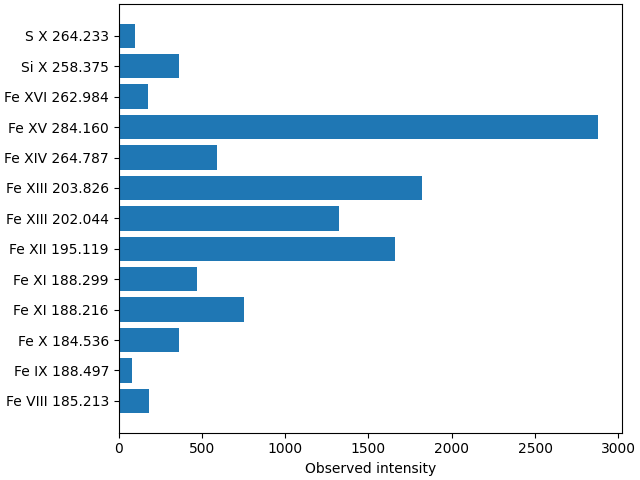
To start with we’ll load a set of line intensities. These have been taken from a single pixel of a fitted Hinode/EIS intensity map, and saved into a netCDF file for easy loading.

line_intensities = xr.open_dataarray(intensity_path)
print(line_intensities)

<xarray.DataArray (Line: 13, Value: 2)>
[26 values with dtype=float64]
Coordinates:
  * Line     (Line) object 'Fe VIII 185.213' 'Fe IX 188.497' ... 'S X 264.233'
  * Value    (Value) object 'Intensity' 'Error'

Now we’ve loaded the intensities, lets do a quick visualisation

fig, ax = plt.subplots(constrained_layout=True)
ax.barh(
    line_intensities.coords["Line"],
    line_intensities.loc[:, "Intensity"],
)
ax.set_xlim(0)
ax.set_xlabel("Observed intensity")

As well as observed intensities, the second ingredient we need for estimating a DEM is the theoretical contribution functions for each observed line. These have been pre-computed and included as sample data. The load_cont_funcs function provides functionality to load these from the saved netCDF file.

cont_funcs = load_cont_funcs(cont_func_path)
for line in cont_funcs:
    print(f"{line}: {cont_funcs[line]}")

Fe VIII 185.213: Fe VIII 185.213 contribution function sampled at 401 temperatures
Fe IX 188.497: Fe IX 188.497 contribution function sampled at 401 temperatures
Fe X 184.536: Fe X 184.536 contribution function sampled at 401 temperatures
Fe XI 188.216: Fe XI 188.216 contribution function sampled at 401 temperatures
Fe XI 188.299: Fe XI 188.299 contribution function sampled at 401 temperatures
Fe XII 195.119: Fe XII 195.119 contribution function sampled at 401 temperatures
Fe XIII 202.044: Fe XIII 202.044 contribution function sampled at 401 temperatures
Fe XIII 203.826: Fe XIII 203.826 contribution function sampled at 401 temperatures
Fe XIV 264.787: Fe XIV 264.787 contribution function sampled at 401 temperatures
Fe XV 284.160: Fe XV 284.160 contribution function sampled at 401 temperatures
Fe XVI 262.984: Fe XVI 262.984 contribution function sampled at 401 temperatures
S X 264.233: S X 264.233 contribution function sampled at 401 temperatures
Si X 258.375: Si X 258.375 contribution function sampled at 401 temperatures

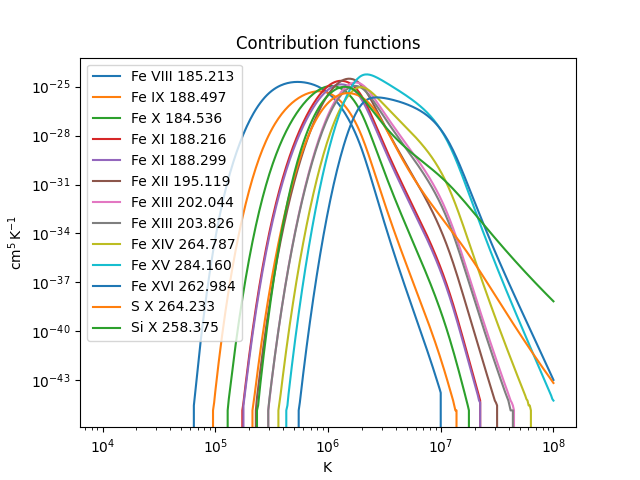
cont_funcs is a dictionary that maps the emission line to a contribution function object. This object stores a pre-computed contribution function at a range of discrete temperature values. Lets do a visualisation of all the contribution functions:

fig, ax = plt.subplots()
for line in cont_funcs:
    ax.plot(cont_funcs[line].temps, cont_funcs[line].values, label=line)

ax.set_xscale("log")
ax.set_yscale("log")
ax.legend()
ax.set_title("Contribution functions")

Having loaded intensities and contribution functions for each emission line, the final preparation step we need to do is create a list EmissionLine objects for each line. This object stores both the observations and theoretical contribution function in a single place for each line.

lines = []
for line in line_intensities.coords["Line"].values:
    if "Fe" not in line:
        # Only use iron lines in the DEM inversion
        continue

    cont_func = cont_funcs[line]
    intensity = line_intensities.loc[line, :]

    line = EmissionLine(
        cont_func,
        intensity_obs=intensity.loc["Intensity"].values,
        sigma_intensity_obs=intensity.loc["Error"].values,
    )
    lines.append(line)

Now we can run the DEM inversion! We have to decide what temperature bins we want to estimate the DEM in. For this example we’ll use 12 bins, with a width of 0.1 MK.

demcmc uses the emcee` package to run the MCMC sampler, and attempt to find the best values of the DEM that match the line intensity observations.

temp_bins = TempBins(10 ** np.arange(5.6, 6.8, 0.1) * u.K)
# Run DEM inversion
dem_result = predict_dem_emcee(lines, temp_bins, nwalkers=50, nsteps=100)
print(dem_result)

You must install the tqdm library to use progress indicators with emcee
<demcmc.dem.DEMOutput object at 0x7f89e32ebf70>

The DEMOutput class has several useful properties. One of those is .samples, which returns the samples of the DEM values at the final step of each MCMC walker.

print(dem_result.samples.shape)
print(dem_result.samples)

(50, 12)
[[2.31706958e+20 7.54520828e+19 3.20328212e+20 5.78238532e+18
  4.30016103e+19 2.17192929e+21 1.59237625e+22 1.24660852e+20
  3.70583767e+21 2.92183190e+21 1.52774317e+21 1.33156501e+21]
 [2.79204456e+20 4.17537719e+19 3.33249873e+20 8.82909530e+19
  2.91462346e+19 1.94143471e+21 1.65106008e+22 1.17900577e+20
  4.01037390e+21 2.39386404e+21 7.60684076e+20 1.13760490e+21]
 [2.38207965e+20 4.70425806e+19 2.44303321e+20 7.23912099e+19
  3.56649237e+19 2.17983409e+21 1.66834527e+22 1.12641562e+20
  3.28331951e+21 3.42113969e+21 2.42046214e+21 6.00731982e+21]
 [2.07956444e+20 6.82777066e+18 2.56458612e+20 7.87769426e+18
  2.71390093e+19 1.48573037e+21 1.70216338e+22 2.82097295e+20
  4.78310036e+21 7.18236654e+20 2.12876025e+21 7.37032665e+19]
 [2.10281704e+20 6.47418037e+19 2.56500060e+20 4.99424586e+18
  4.35992634e+19 2.52358095e+21 1.61747048e+22 1.31354095e+20
  3.57708093e+21 3.29076021e+21 2.16089902e+21 2.79457872e+21]
 [2.27399427e+20 9.70064110e+19 3.13189146e+20 3.53363540e+19
  4.54033445e+19 2.81755178e+21 1.54469270e+22 1.85784398e+19
  2.88224478e+21 4.54360001e+21 2.00837877e+18 5.30019747e+21]
 [1.94058987e+20 7.12993724e+19 2.66700847e+20 2.16637014e+19
  3.88030447e+19 2.68849785e+21 1.52963109e+22 6.16454471e+19
  3.01399263e+21 3.81077333e+21 2.63352713e+21 5.19124602e+21]
 [2.49425512e+20 6.78934813e+19 3.42411009e+20 4.74415287e+19
  3.34142359e+19 2.12412580e+21 1.63547030e+22 1.63365304e+19
  3.19924889e+21 2.78089795e+21 2.00665262e+21 5.51244184e+21]
 [3.35041652e+20 4.03094341e+19 4.32390974e+20 1.32263106e+20
  2.04911441e+19 7.92222480e+20 1.84454982e+22 2.18888736e+19
  3.48754816e+21 3.51102899e+21 5.71876068e+20 4.97273055e+21]
 [2.65109971e+20 8.25269624e+19 3.73855958e+20 5.27767219e+19
  3.25051935e+19 1.80682491e+21 1.63549974e+22 2.66077682e+19
  3.70591397e+21 3.04397750e+21 2.23499021e+21 3.29949325e+21]
 [2.27060557e+20 3.88933307e+19 2.64237745e+20 5.46527297e+19
  3.20748832e+19 2.24793303e+21 1.56295278e+22 1.79406355e+20
  4.06955109e+21 3.09743117e+21 8.85045675e+20 5.46154698e+20]
 [2.52794583e+20 6.99158362e+19 3.42574393e+20 2.57755506e+19
  2.93443881e+19 1.57665242e+21 1.75604661e+22 2.61478049e+19
  3.48110787e+21 3.24821227e+21 2.71085367e+21 5.73148462e+21]
 [2.45387877e+20 2.47095973e+19 2.54364816e+20 1.04387486e+20
  2.61069298e+19 2.66459563e+21 1.57254490e+22 1.99096241e+20
  4.45669423e+21 3.75913295e+21 1.74387285e+21 5.37750846e+20]
 [2.43573657e+20 4.52995275e+19 2.70069340e+20 7.61003723e+19
  3.16781462e+19 2.33251327e+21 1.61885226e+22 7.83302337e+19
  2.83803622e+21 2.81551479e+21 4.37839338e+21 7.73273796e+21]
 [2.89649525e+20 9.54761066e+18 2.71009015e+20 1.39987427e+20
  2.27074867e+19 2.65830126e+21 1.65083447e+22 1.71406993e+20
  3.74492319e+21 1.44281117e+21 1.67438931e+21 2.54894029e+21]
 [2.10341339e+20 8.53984297e+19 2.91999676e+20 2.70412642e+19
  4.10079953e+19 2.78990860e+21 1.51428755e+22 2.87398058e+19
  3.23168718e+21 5.59678897e+21 1.54923963e+21 4.00488968e+21]
 [3.10767321e+20 8.82211771e+18 3.14013032e+20 2.20408728e+20
  1.03110591e+19 2.29392775e+21 1.54663317e+22 9.68376312e+19
  3.64845669e+21 2.36445300e+21 4.06493260e+21 6.23024220e+21]
 [2.51100307e+20 9.25279940e+19 3.28481978e+20 3.69037008e+19
  4.15276988e+19 2.22521613e+21 1.66062357e+22 7.62373181e+18
  3.07311203e+21 4.79839580e+21 8.16274637e+20 5.54883507e+21]
 [1.85269394e+20 5.59579106e+19 2.09900197e+20 1.72287664e+19
  4.44216139e+19 3.29628274e+21 1.51920314e+22 8.95048500e+19
  2.50605282e+21 4.31406821e+21 1.41297390e+21 7.89326807e+21]
 [2.27558687e+20 6.69408339e+19 3.22045032e+20 2.25455813e+19
  3.50828399e+19 2.03418528e+21 1.62729586e+22 1.98368981e+19
  3.04742429e+21 3.16210316e+21 1.98293420e+21 5.02058281e+21]
 [2.61302711e+20 2.74790915e+19 2.78526899e+20 1.37773269e+20
  2.25029419e+19 2.44881383e+21 1.54143796e+22 1.67395416e+20
  4.10440148e+21 2.65924415e+21 2.44473232e+21 2.67054068e+21]
 [2.29580318e+20 6.04720568e+19 2.99318969e+20 6.76507741e+19
  3.69875033e+19 2.86344502e+21 1.53618295e+22 1.04570888e+20
  3.72057820e+21 4.15119226e+21 2.37772557e+21 1.51188235e+21]
 [2.55481149e+20 6.04307587e+19 3.25445469e+20 5.71589099e+18
  4.19186457e+19 1.60507561e+21 1.67314566e+22 1.21544553e+20
  3.25832297e+21 1.29925877e+21 3.31053083e+21 4.23219987e+21]
 [2.74651317e+20 3.34343887e+19 3.02633239e+20 1.28266866e+20
  2.68379433e+19 2.61183280e+21 1.57082415e+22 1.13695864e+20
  3.58282324e+21 2.81380630e+21 1.68357658e+21 3.14277565e+21]
 [2.59855905e+20 4.30961216e+19 2.69020822e+20 9.03676893e+19
  3.20526677e+19 2.23487609e+21 1.62182689e+22 1.46999730e+20
  3.89398785e+21 4.73083283e+21 6.49622616e+20 2.34803434e+21]
 [2.17628120e+20 3.53544142e+19 2.82223055e+20 5.80905092e+19
  3.11186799e+19 2.84801362e+21 1.61631264e+22 1.31283276e+20
  4.07540866e+21 2.43854481e+21 2.53869663e+21 2.90403415e+21]
 [1.91502763e+20 6.17796217e+19 2.66142216e+20 2.29404219e+19
  3.64359908e+19 2.38816071e+21 1.63321454e+22 6.91974961e+19
  3.37085924e+21 2.88004075e+21 3.75229131e+21 6.14056542e+21]
 [1.98741330e+20 6.80917281e+19 2.69288562e+20 1.53963026e+19
  3.64648648e+19 2.70392490e+21 1.59738716e+22 5.68445068e+19
  3.03095042e+21 3.86440798e+21 3.39502520e+21 6.91128547e+21]
 [2.79971986e+20 3.49159728e+19 3.09646028e+20 9.91431107e+19
  2.43392042e+19 1.83125546e+21 1.71358671e+22 1.07558626e+20
  3.85842102e+21 2.35994486e+21 2.65764669e+21 3.65009476e+21]
 [2.30994040e+20 5.13449314e+19 2.57147207e+20 6.70775883e+19
  3.17051785e+19 2.42715087e+21 1.58710989e+22 1.25939459e+20
  3.69617088e+21 4.34720028e+21 2.85308506e+21 4.13862818e+21]
 [2.39342759e+20 4.59467320e+19 2.24856475e+20 1.04738715e+20
  3.50328969e+19 3.44069203e+21 1.49419300e+22 1.49722046e+20
  3.54675757e+21 3.77357987e+21 4.68811249e+20 2.24700524e+21]
 [2.25344934e+20 4.15459750e+19 2.55557322e+20 6.74564584e+19
  3.64399796e+19 2.69258588e+21 1.56033453e+22 1.82766702e+20
  4.01350054e+21 4.91937150e+21 7.04179920e+20 1.42142115e+21]
 [2.76679901e+20 3.07309893e+19 3.26407319e+20 1.04533817e+20
  2.42520220e+19 1.82924405e+21 1.68083553e+22 1.40055806e+20
  4.16423206e+21 1.77445108e+20 3.19690441e+21 1.62503781e+21]
 [2.91569616e+20 3.95557856e+19 3.02290758e+20 9.28783528e+19
  2.87659142e+19 1.65694427e+21 1.70145080e+22 1.37787877e+20
  4.13128230e+21 3.67188319e+21 3.48161973e+20 8.16421698e+20]
 [2.49312874e+20 8.64810907e+19 3.27351165e+20 5.22507585e+19
  3.73170435e+19 2.36441074e+21 1.59349513e+22 5.78548305e+19
  3.70488386e+21 4.43589434e+21 6.96021030e+20 2.63806539e+21]
 [1.71788824e+20 5.63010429e+19 2.07804237e+20 1.01745274e+19
  4.06137694e+19 2.47831811e+21 1.58789585e+22 1.66019720e+20
  3.61004330e+21 3.15376653e+21 4.02234994e+21 4.49563824e+21]
 [2.50997132e+20 4.87594466e+19 1.90059137e+20 4.70973834e+19
  4.21106208e+19 1.99689828e+21 1.70872014e+22 2.69592638e+20
  3.04349092e+21 3.20063431e+21 2.80379020e+21 6.30481942e+21]
 [1.71538403e+20 4.73302878e+19 2.31862357e+20 3.26713064e+19
  3.70947558e+19 3.26598190e+21 1.51891288e+22 1.68868785e+20
  4.14910646e+21 3.71804781e+21 1.73575528e+21 2.10987054e+21]
 [2.05246043e+20 5.87124228e+19 2.26541777e+20 4.21445226e+19
  3.89137274e+19 2.79709657e+21 1.54355214e+22 1.66859584e+20
  3.70239842e+21 4.51046526e+21 1.86965411e+21 2.77810274e+21]
 [2.30480952e+20 5.45322375e+19 2.64734884e+20 1.92023230e+19
  3.91493340e+19 2.01820344e+21 1.62890830e+22 1.51707519e+20
  3.50986620e+21 3.10014334e+21 2.55792145e+21 3.80473001e+21]
 [2.71152783e+20 5.98780559e+19 3.64655753e+20 9.63450625e+19
  2.61775185e+19 1.96630837e+21 1.65381806e+22 3.79348488e+19
  3.93950778e+21 2.88030899e+21 2.47350956e+21 2.14684569e+21]
 [3.00106422e+20 4.43606526e+19 2.18069228e+20 7.36990519e+19
  4.15823590e+19 1.52894425e+21 1.71394440e+22 3.25405265e+20
  3.59095179e+21 3.11775822e+21 1.68611888e+21 1.21573368e+21]
 [2.95459755e+20 4.29641321e+19 3.59971809e+20 2.06131817e+20
  2.04005408e+19 3.45988663e+21 1.48369869e+22 7.43637564e+19
  3.87862101e+21 2.51177911e+21 3.83568770e+21 3.63190467e+21]
 [2.82018627e+20 5.85141950e+19 3.52989063e+20 5.85836373e+19
  2.99634502e+19 1.06900775e+21 1.71229587e+22 4.17981044e+19
  3.32197926e+21 1.27536847e+21 3.11866277e+21 5.35859302e+21]
 [2.34018922e+20 4.91453664e+19 2.50040503e+20 3.26250479e+19
  3.87569779e+19 1.60309344e+21 1.64971938e+22 2.50903843e+20
  4.04123635e+21 1.30114854e+21 3.89911968e+21 2.40914192e+21]
 [2.32032866e+20 1.57235391e+19 2.16988961e+20 1.20186563e+20
  3.04411196e+19 3.27010180e+21 1.50744326e+22 1.84925387e+20
  3.85053797e+21 3.52559497e+21 1.66691306e+21 3.16568610e+21]
 [2.58918065e+20 4.48816563e+19 3.23583924e+20 7.26353596e+19
  2.58474320e+19 1.67201248e+21 1.66756300e+22 1.58722336e+20
  4.32073221e+21 1.95054946e+20 3.78089423e+21 1.19746702e+21]
 [2.02421984e+20 4.61327787e+19 2.52911026e+20 4.66634555e+19
  2.99920743e+19 2.69933803e+21 1.60103773e+22 9.43345996e+19
  3.27422570e+21 2.56905806e+21 3.81153292e+21 6.66012032e+21]
 [2.51472527e+20 4.79257650e+19 2.80219126e+20 7.76581712e+19
  3.01570456e+19 2.03463331e+21 1.61188402e+22 1.42783235e+20
  3.79282908e+21 2.91457768e+21 2.96604442e+21 3.19050088e+21]
 [2.53955488e+20 8.78167030e+19 2.67222045e+20 4.96599632e+19
  4.17146636e+19 2.42137340e+21 1.61342472e+22 2.89729271e+19
  2.82802815e+21 5.08857444e+21 7.30289421e+20 5.44140360e+21]] 1 / cm5

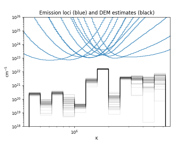
To visualise the result, we can plot the final samples, and then plot the emission loci on the same axes. The emission loci give an upper bound on the DEM.

fig, ax = plt.subplots()

dem_result.plot_final_samples(ax)
plot_emission_loci(lines, ax, color="tab:blue")

ax.set_xscale("log")
ax.set_yscale("log")
ax.set_xlim(temp_bins.min * 0.9, temp_bins.max * 1.1)
ax.set_ylim(1e18 * u.cm**-5, 1e26 * u.cm**-5)
ax.set_title("Emission loci (blue) and DEM estimates (black)")

Finally, we should check if the MCMC walker converged or not.

chain = dem_result.sampler.get_chain()
nsamplers = chain.shape[1]
nparams = chain.shape[2]

fig, axs = plt.subplots(nrows=nparams, sharex=True, figsize=(6, 20))

for ax, param in zip(axs, range(chain.shape[2])):
    for sampler in range(chain.shape[1]):
        ax.plot(chain[:, sampler, param], color="tab:blue", alpha=0.1)

    # Plot average of each walker at each step
    ax.plot(np.mean(chain[:, :, param], axis=1), color="k")

    ax.set_yscale("log")
    ax.margins(x=0)
    ax.xaxis.grid()

fig.subplots_adjust(hspace=0)
axs[0].set_title("Parameter estimates as a function of MCMC step")

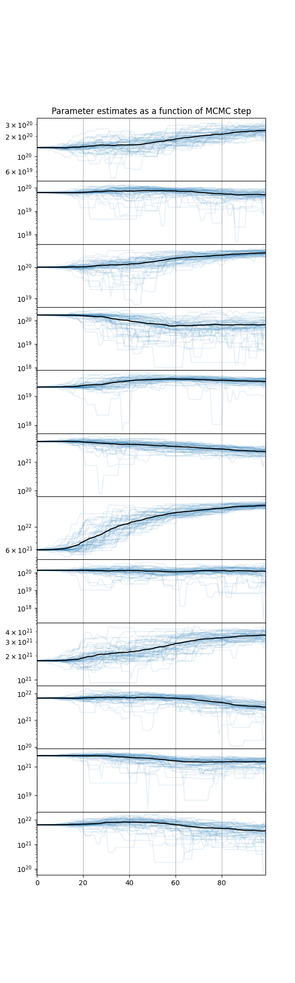
There are still large scale variations going on for each parameter, so clearly the MCMC run has not converged. When running demcmc yourself make sure to set an appropriate number of walkers and steps so the parameter estimates converge!

plt.show()